Modelling acoustic spatial capture-recapture data with acre

Set up

To participate in this workshop you need to install two packages, neither of which are currently available on CRAN. The easiest way to install these packages is to first install the devtools package, and then run the following code, although Windows users will need Rtools installed first. If you install Rtools, or have to reinstall either acre or acreworkshop, then restart your R session before continuing.

library(devtools)
install_github("b-steve/acre", ref = "perth-workshop")
install_github("b-steve/acreworkshop")

Once you’ve installed the packages, load them into your R session.

library(acre)
library(acreworkshop)

A quick disclaimer

The acre package is still under development, so there’s a good chance something will go wrong! If you think you have fallen victim to a bug, let Ben know, and we can try to help you out and fix it later on. The documentation is not complete, so if you’re stuck with how to use a function then feel free to ask us any questions.

If you have any suggestions to improve the package then let us know: we’d love to hear them.

Introduction and background

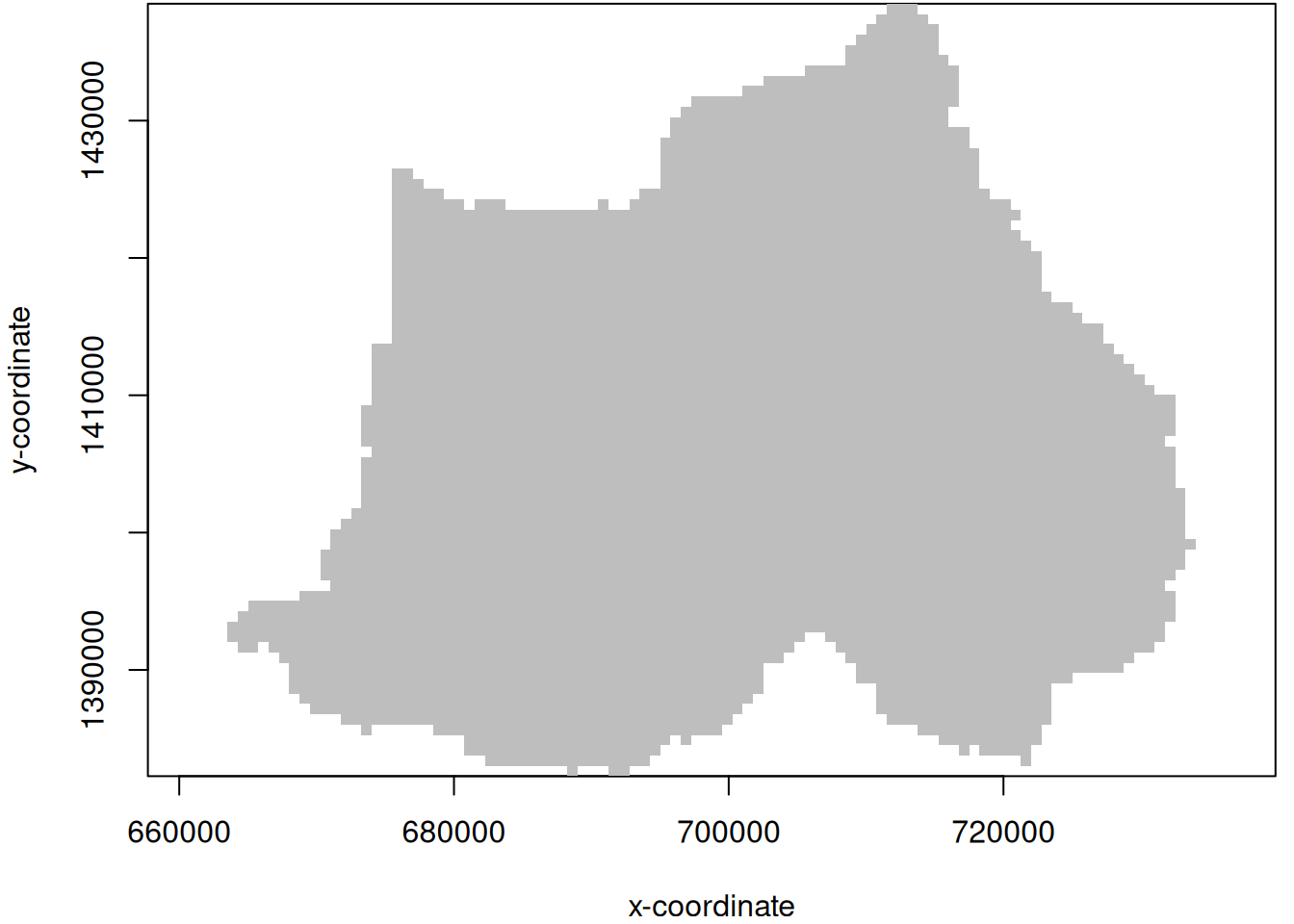
Congratulations! You have just been appointed as conservation manager of the southern yellow-cheeked crested gibbon (Nomascus gabriallae) in Phnom Prich Wildlife Sanctuary (PPWS), Cambodia (Figure 1). Exactly why they have appointed someone who lives so far away is a bit of a mystery, but you decide to take on the responsibilities nonetheless.

Figure 1: A map of Phnom Prich Wildlife Sanctuary. The x- and y-coordinates are in metres.

Nomascus gabriallae is currently listed as an endangered species by the IUCN. Worldwide, gibbons are threatened by habitat loss from expansions in industrial agriculture, and are also hunted in Cambodia for food, for biomedical purposes including traditional medicine, and for the pet trade. Gibbon populations are important because studying them can help us understand our own evolutionary history, and also understand emerging diseases that affect both humans and primates. They also play a role in seed dispersal in forests, and have cultural importance in the local region.

It is your job to estimate density and distribution of Nomascus gabriallae in PPWS: how many groups are there, and where do they live?¹ To achieve this goal, you will conduct an acoustic survey: you will select 18 locations throughout the park, and at each, your team will establish three listening posts, with a distance of 1 km between adjacent posts. This is a common design for acoustic surveys of gibbons—see Kidney et al. (2016) and McGrath et al. (2023), for example. In this analysis we will assume each group calls once per day, in the morning. Things are a little more complicated in reality, for example because not all gibbon groups call on any given day—but we will ignore these issues for the purposes of this exercise.

Each set of three listening posts will collect acoustic spatial capture-recapture (SCR) data. When a gibbon group calls it can be detected by the listening posts, and when a detection occurs, the fieldworkers at the listening post use a compass to estimate the direction from which the sound originated. We can then use an SCR model to estimate density and distribution in PPWS using the R package acre.

But first, you need to gain a better understanding of the wildlife sanctuary itself. Gibbon population density can vary over space in response to various environmental covariates, which in this case may be the following:

• Canopy height: Your biologist collaborators suspect that gibbons prefer to live in taller trees, so regions of PPWS with higher canopies are more likely to support larger numbers of gibbons. Canopy height is measured in metres.
• Forest type: PPWS is covered in forest, but the type of forest varies between evergreen and deciduous forest. It’s possible gibbons will prefer one to the other.
• Elevation: Gibbons may prefer living at high elevations, low elevations, or somewhere in between. Elevation is measured in metres above sea level.
• Villages: It is well known that gibbons try to avoid humans, so we might expect gibbon population density to be low at locations close to villages.

Question 1

Unfortunately it’s impossible to observe the covariates canopy height, forest type, and elevation at every location in PPWS: you don’t have the budget to measure every single tree. Nevertheless, you do need to know how these covariates vary over the whole region. Unfortunately there are no good ways to obtain these measurements from satellite data, nor are there GIS products available for the region². Yes, you guessed it: it will involve leg work. Your team’s leg work!

To achieve this, you have the budget to select 24 locations to deploy fieldworkers to measure these covariates, and then you will rely on a statistical method known as spatial interpolation to fill in the gaps.

First, run the following line of code in R. A plot will appear, and you can click on it to select the locations at which to measure these covariates. Then you can fly to Cambodia and deploy your team.

cov.df <- measure.covariates()

Don’t stress too much about the specific locations you select. There isn’t a particular right answer, although you can probably think of some strategies that are worth avoiding.

Once your data have been collected, take a look at the cov.df data frame to see the data you have collected. You can also create plots of the covariates using the following R code. Replace "var" with the name of a column in cov.df to take a look at different variables.

plotcov(cov.df, "var")

Question 2

As you will have seen from your plots, there are large regions of PPWS at which you do not currently have covariate values. To carry out spatial interpolation on your data, you can use the following line of code:

interpolated.df <- interpolate.covs(cov.df)

See what happens when you create plots of covariates again, but using interpolated.df at the first argument instead of cov.df.

Note

We do not have to carry out spatial interpolation for our distance to village covariate: we know where the villages are, and so we can calculate the exact distance to the nearest village for any location in PPWS instead. The village locations can be found in the data frame villages.df.

Question 3

Now it is time to conduct the acoustic surveys. Your first job is to select the locations at which each of the 18 sets of three listening posts will be deployed. We refer to each of these 18 sites as a session. It’s not necessary, but you might want to consider the plots of covariates from the previous question when making up your mind.

Run the following line of code to carry out your acoustic surveys:

survey.data <- conduct.survey()

The survey.data object is a list with two components:

• survey.data$traps contains the locations at which you decided to deploy your listening posts.
• survey.data$captures contains detection data collected on the surveys. See if you can figure out what each column means.

Question 4

It’s finally time to use the acre package. First, load it up, if you haven’t already:

library(acre)

So far, you have collected data from a variety of sources: you have covariate information in cov.df, you have village locations in villages.df, you have listening post locations in survey.data$traps, and you have detection data in survey.data$captures.

The first step is to combine all of these data sources together into an R object using the read.acre() function. It is your job to create this object. There are five arguments you’ll need to use:

1. captures: the data frame with the detection data.
2. traps: the object with the listening post locations.
3. control.mask: you need to specify the maximum distance at which you can possibly detect a gibbon. In this case, the maximum feasible distance is \(3\,000\) m. Use control.mask = list(buffer = 3000) for this argument.
   
4. loc.cov: a data frame with columns x and y, specifying locations at which spatial covariates have been measured, and then a further column for each spatial covariates themselves. For this step you should provide the data frame containing the measured covariate values, rather than the interpolated values. The function will complete the interpolation for you.
5. dist.cov: a data frame containing locations of objects of interest, from which you want to construct a spatial covariate for the distance to the nearest object. This needs to be a list, where each component name relates to the type of object, and the component itself is a data frame with columns named xand y specifying the locations of these objects. In this case, we just have to obtain the distance to the nearest vilage for each point in PPWS, so you can use dist.cov = list(village = villages.df).

The acre package can create plots of your data for you. Can you guess what is being shown when you run the following?

Note

The data object is that returned by read.acre().

## Press return many times after initial plotting.
plot(data, type = "capt")
## Press return a few times. What happens if you change 'session'?
plot(data, type = "covariates", session = 1) 

Question 5

Now it’s time to fit some models! Once you have a data object from read.acre(), this is straightforward. You can fit a default model like this:

fit1 <- fit.acre(data)

You can ignore the output outer mgc: ... during model fitting.

To inspect model output, you can try using the following functions. See if you can figure out what the output means from each:

summary(fit1)
## What happens if you change 'session'?
plot(fit1, type = "Dsurf", session = 1) 
plot(fit1, type = "Dsurf", new.data = ppws)
plot(fit1, type = "detfn")
AIC(fit1)

Question 6

Experiment with fitting more sophisticated models using additional arguments. Here are a couple of ideas.

First, the detection function can be selected with the detfn argument. The default is detfn = "hn", corresponding to the halfnormal detection function. To adjust the detection function, you can set the detfn argument to "hhn" for the hazard halfnormal function or "th" for the threshold detection function.

Second, by default, a homogeneous density model is fitted, so that estimated density is the same across the whole sanctuary. To allow density to vary with spatial covariates, you can use the model argument like this:

fit2 <- fit.acre(data, model = list(D = ~ var1 + var2))

You can also allow other model parameters (e.g., detection function parameters) to vary with covariates, but we won’t explore that in this workshop.

Note

Here are some additional notes on fitting more sophisticated inhomogeneous density models. Don’t feel like you need to explore these ideas, but they’re available to you if you have time, and you’d like to give them a try.

• You can use x and y to allow density to vary with the x and y coordinates in PPWS.
• You can use any of the regular formula features available in functions like lm(). Here are some examples:
  • Interaction terms, for example using var1*var2.
  • Polynomial terms, for example using poly(), or var + I(var^2).
    
  • Any other variable transformations using I(), for example using I(ifelse(var > 10, "large", "small")) to create a categorical variable from a continuous variable.
• You can use the s() function from mgcv to fit unpenalised splines. Because the splines are unpenalised, you need to be careful about setting the k parameter: too large and you’ll overfit, too low and you’ll underfit.

Question 7

? Competition time ?

Because these are simulated data, I know exactly how gibbon density varies throughout the wildlife sanctuary. There is a prize for whoever’s model does the best job!

Decide which of your models you like best so that you can enter it in our competition. Name the object fit.final, and run the following line of code:

save(fit.final, file = "firstname-lastname.RData")

Make sure to replace "firstname-lastname" with your actual first and last names, and don’t ignore the hyphen. For example, I would do the following:

save(fit.final, file = "ben-stevenson.RData")

In my case, a file named ben-stevenson.RData will be created on my hard drive, within my R working directory. Find this file on your system and upload it using this link. If you’re not sure what your R working directory is, then run getwd() to find out.

In case you’re interested…

The density of southern yellow-cheeked crested gibbon (Nomascus gabriallae) groups in this simulated example was quite a bit higher than they actually are in PPWS. In reality, there are almost no gibbons throughout most of the sanctuary but there are a couple of small pockets of high-density forest.

However, population density in this example is roughly similar to that of the closely related northern yellow-cheeked crested gibbon (Nomascus annamensis) in Veun Sai-Seim Pang National Park, also in Cambodia.

References

Kidney, D., B. Rawson, D. L. Borchers, B. C. Stevenson, T. A. Marques, and L. Thomas. 2016. “An Efficient Acoustic Density Estimation Method with Human Detectors Applied to Gibbons in Cambodia.” PLoS ONE 11: e0155066.

McGrath, S., J. Liu, B. C. Stevenson, and A. M. Behie. 2023. “Density and Population Size Estimates of the Endangered Northern Yellow-Cheeked Crested Gibbon Nomascus Annamensis in Selectively Logged Veun Sai-Siem Pang National Park in Cambodia Using Acoustic Spatial Capture-Recapture Methods.” PLoS ONE 18: e0292386.

Footnotes

1. Note that the data you will be using in this exercise are simulated and do not truly reflect the spatial covariates, nor the density and distribution of Nomascus gabriallae in Phnom Prich Wildlife Sanctuary, but the challenges you will face here are similar to those from a real data set.

2. This sentence isn’t quite true in reality, but let’s assume it is true for the purposes of this exercise.